
How to use array formulas to eliminate unnecessary intermediate calculations.
Often times if you are making a spreadsheet with more complicated calculations, you will have rows of data used for intermediate calculations before you get to the actual result. In fact it is not uncommon for me to have multiple sheets worth of this. You then have to hide the rows or sheets to keep things from getting messy.
However, using array formulas you can often times eliminate most or all of those intermediate calculations. Not only does this make your spreadsheet less messy, but it can help speed your spreadsheet up considerably as well. The example below will show you how to do this.
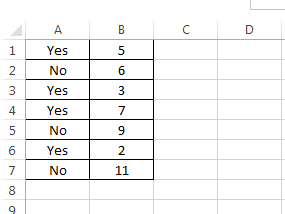
In the example below, I would like to calulate the maximum value in column B for which there is a corresponding "Yes" in column A.
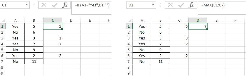
One way I could do this is by making column C into an intermediate column that eliminates the numbers with "No" next to them. The I could find the maximum value of just those remaining numbers. I would then hide column C when I was done.
But I could also use an array formula instead, thus eliminating the need for column C entirely. The way this works is by making your single cell references into the entire ranges. You then press Ctrl-Shift-Enter when you are done, which is how you get those fancy brackets around it, which is what specifies that you have an array formula.
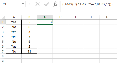
Note: If I were to reference A:A and B:B instead of A1:A7 and B1:B7, then I could input as much data as I wanted and the formula would work on the entire thing, whereas the intermediate column would have to be copied down to match how much data I had each time I added some. Setting up your spreadsheet with array formulas like A:A and B:B works especially well when combined with the automatic borders trick because the user can enter as much data as they want without having to worry about what's going on in the background.